Is the pattern real? R², p-values and prediction bands on a Power BI scatter chart

A scatter chart is the fastest way to see whether two things move together: revenue growth and margin, price and volume, tenure and pay, throughput and defects. It is also the easiest chart to over-read. The eye finds a line in almost any cloud of points, and a trend line drawn through the cloud makes it look official.

Three numbers decide whether the line deserves attention: R², the p-value and the width of the prediction band. Below: the data shape a Power BI scatter needs, the DAX for each number, how to read them, and a checklist for the next scatter in a report.

First, the single dot

The most common scatter question on the forums is not statistical at all: "I put two measures on X and Y and get one dot." A measure is evaluated in the filter context of each point, and a point is defined by the field in the Values well of the built-in scatter (Details in older versions). With nothing there, there is one context, the whole table, and so one dot.

Put the entity you want to compare in that well: Customer, Site, Rep, Product. Each value becomes a point, and X and Y are evaluated per value. If you put a column instead of a measure on X, Power BI aggregates it (sum by default), which is rarely what a scatter wants; use a measure that means something per entity, such as Revenue Growth % or Gross Margin %.

For the Helios Manufacturing customer portfolio, the model is a sales fact table with Sales[Customer], Sales[OrderDate], Sales[Amount] and Sales[Cost], a customer dimension and a marked date table:

Revenue = SUM ( Sales[Amount] )

Revenue PY =
CALCULATE ( [Revenue], SAMEPERIODLASTYEAR ( 'Date'[Date] ) )

Revenue Growth % =
DIVIDE ( [Revenue] - [Revenue PY], ABS ( [Revenue PY] ) )

Gross Margin % =
DIVIDE ( [Revenue] - SUM ( Sales[Cost] ), [Revenue] )

Start with the picture, then the numbers

Before reading any statistic, look for the things that break statistics: a few points far from the rest, two separate groups, a curve rather than a line. One large customer in a corner can create a correlation that the other two hundred do not share. A cloud made of two clusters can show a strong overall trend while each cluster on its own has none.

Pearson r and its p-value in DAX

Pearson's r measures how well a straight line describes the cloud, from -1 to 1. In DAX, build the table of points once and compute r over it:

Correlation r =
VAR Pts =
    FILTER (
        ADDCOLUMNS (
            VALUES ( Customer[Customer] ),
            "@x", [Revenue Growth %],
            "@y", [Gross Margin %]
        ),
        NOT ISBLANK ( [@x] ) && NOT ISBLANK ( [@y] )
    )
VAR MeanX = AVERAGEX ( Pts, [@x] )
VAR MeanY = AVERAGEX ( Pts, [@y] )
VAR Sxy = SUMX ( Pts, ( [@x] - MeanX ) * ( [@y] - MeanY ) )
VAR Sxx = SUMX ( Pts, ( [@x] - MeanX ) ^ 2 )
VAR Syy = SUMX ( Pts, ( [@y] - MeanY ) ^ 2 )
RETURN
    DIVIDE ( Sxy, SQRT ( Sxx * Syy ) )

The FILTER matters: a customer without last year's revenue has a blank growth and must leave both sums, not enter them as zero.

The p-value answers: if there were no relationship at all, how often would a sample this size show a correlation at least this strong? It comes from a t statistic with n - 2 degrees of freedom:

Correlation p =
VAR Pts = …  -- the same points table as in Correlation r
VAR n = COUNTROWS ( Pts )
VAR r = [Correlation r]
VAR t = r * SQRT ( DIVIDE ( n - 2, 1 - r ^ 2 ) )
RETURN
    IF ( n >= 3 && ABS ( r ) < 1, T.DIST.2T ( ABS ( t ), n - 2 ) )

Read it carefully. A p-value of 0.005 says the pattern is unlikely to be noise. It does not say the effect is big: with 10,000 points even a tiny, useless correlation gets a small p-value. With twelve points a real effect can miss 0.05. That is why r and p should always be shown next to n.

Pearson's r also reacts to outliers and only measures straight lines. When the relationship rises steadily but not in a straight line, or a few extreme values dominate, the rank-based Spearman ρ and Kendall τ-b are the safer reading.

R² and the trend line with LINESTX

LINESTX fits a least-squares line over a table and returns the slope, intercept, R² and standard errors in one row:

Trend R² =
VAR Pts = …  -- the same points table as in Correlation r
RETURN
    MAXX ( LINESTX ( Pts, [@y], [@x] ), [CoefficientOfDetermination] )

Trend Slope =
VAR Pts = …  -- the same points table as in Correlation r
RETURN
    MAXX ( LINESTX ( Pts, [@y], [@x] ), [Slope1] )

An R² of 0.13 means the line accounts for 13 % of the variation in margin; the other 87 % is everything the line does not capture. It says nothing about cause. A small R² can still matter when the slope is large and reliable, and a high R² on a dozen points can be luck. For a straight line with one X, R² is simply r squared, so the two measures should agree; if they do not, the two point tables differ.

Confidence band or prediction band?

This is the number most reports leave out. Around a fitted line there are two bands, and they answer different questions:

The confidence band shows where the average Y at a given X probably lies. With many points it gets narrow, because the average is well known.
The prediction band shows where a single new point probably lands. It stays wide when the data is noisy, however many points there are.

Both come from the same formula. With s the residual standard error, n the number of points, x̄ the mean of X and Sxx the sum of squared deviations of X, the 95 % bands at a value x are

ŷ ± t · s · √(1/n + (x − x̄)² / Sxx) for the confidence band, and ŷ ± t · s · √(1 + 1/n + (x − x̄)² / Sxx) for the prediction band,

where t is the 97.5 % quantile of the t distribution with n - 2 degrees of freedom (T.INV.2T ( 0.05, n - 2 ) in DAX). LINESTX returns s as StandardError. Both bands widen away from the middle of the data, because the slope is least certain at the ends.

If you are pricing a new deal, the prediction band is the question you are actually asking: at this price, what volume is normal? A deal outside the 95 % prediction band is worth a look; a deal inside it is ordinary, however far it sits from the line.

Pick the fit for the shape, not for the R²

A cubic curve always has a higher R² than a straight line, because it has more freedom, not because it is right. Adjusted R² penalises the extra terms, and the p-value of each coefficient says whether a term earns its place: if the quadratic term's p-value is 0.4, the curve is not earning its keep. Logarithmic and power fits often suit price and volume data; on log axes they look straight. A smoother such as LOESS is a useful guide through a cloud but carries no p-values, so do not read significance into it.

A checklist before anyone acts on a trend line

Put the entity in Values (or Details), and check that each point is the thing you mean.
Look for outliers and groups before reading any number.
Read R² next to n, never alone.
Read the p-value as "could this be noise?", and the size of r as "how strong?".
Use the prediction band to judge single points, the confidence band to judge the average.
Prefer the simplest fit whose extra terms have small p-values.
Correlation is not cause. The chart tells you where to look, not why.

Doing it with SmartVisuals Scatter & Bubble

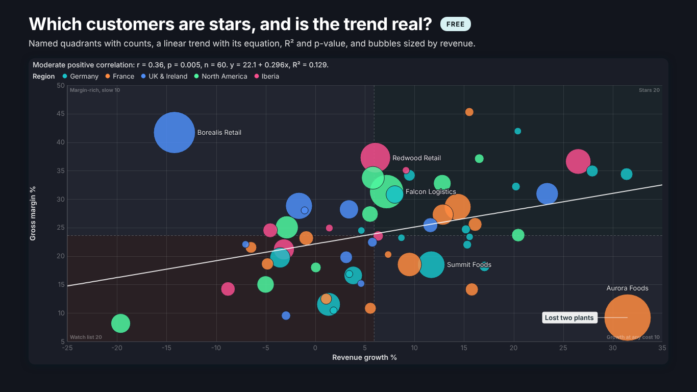
SmartVisuals Scatter & Bubble states the answer in its caption, in one sentence such as "Moderate positive correlation: r = 0.36, p = 0.005, n = 60. y = 22.1 + 0.296x, R² = 0.129." Put Customer in Details, the two measures in X and Y and, for a bubble chart, Revenue in Size; the trend stays on when you add Size, because size is a display choice, not a reason to drop the fit. The free version covers steps 1 to 4: the linear trend with its equation and R², Pearson r with its p-value and an optional 95 % confidence interval, named quadrants with counts, a ring on points far from the trend, and up to 10,000 points.

Premium adds confidence and prediction bands at 90, 95 or 99 %, quadratic, cubic, logarithmic, exponential, power and LOESS fits, a coefficient table with standard errors and p-values, Spearman and Kendall, influence diagnostics that say why a point bends the line, movement against the prior period and up to 100,000 points, for $1.99 per user per month or $19 per user per year. Every statistic is compared with scipy and statsmodels in an automated test suite, every Premium feature previews in full while you edit, and nothing leaves the report. The visual has been submitted to Microsoft Marketplace and is not published yet; the product page will link to the listing once it is live.